
A common way to understand a system is to make a small change to the system, say raise the temperature or pH of the solution, or introduce a new molecule to the sample, and then monitor how this change effects a property of the sample. These properties are often measured with analytical techniques like spectroscopy. This monitoring can be as simple as collecting a single data point before and after the perturbation to the system, or more often, the sample is monitored over time, with several data points collected.
Depending on how slowly the measured property of the system changes as a result of alteration of the system, it may be necessary to collect hundreds or even thousands of data points, otherwise known as scans, of the system. Once this data is collected, however, it can be intimidating to work with such a vast amount of data. Often times, each scan needs to be fit to extract out the necessary information about the systems. Processing each scan individually can be tiresome and leaves lots of room for error. Further, there are often bits of the data that we don't care about, like headers and footers, or the data is stored as strings of characters rather than numbers, making it difficult to process.
To address this problem, it makes the most sense to work with the data as a whole, and to do this a programming language is necessary. This type of data is essentially a huge table, and Python has several libraries which places Python in an exceptional place to work with this data simply and efficently.
Here I will illustrate how to generally work with such data as well as utilize the NumPy and Pandas libraries that Python has to offer. To do so, I crafted a jupyter notebook which resides in my blog repository. This notebook illustrates some of the things discussed here, as well as serves as a reference for working with these libraries.
The sample dataset I will use to illustrate these ideas is from a fluorescence spectroscopy experiment. The sample dataset can be found in my repository . This is a great model experiment type to work with because, generally, the fluorescence spectra is simple, consisting of a single gaussian, or several gaussian peaks. If we make a small change to a system which results in the slow shifting of a fluouresence peak over time, we can monitor this shift by continually scanning the sample, and after each scan saving the spectra to the next column in a table.
The best way to visualize this raw data is by using a Pandas dataframe. If you read my blog post about the data array data type, you will know that I am partial to using NumPy data arrays to work with data. However, when it comes to visualizing and indexing arrays of this type, where we have several scans with header names, it is very helpful to use a Pandas dataframe.
The NumPy data array is called an "ndarray", which stands for N-dimensional array. This means that numpy arrays can have "N" dimensions and is not limited to a 2D array. This is helpful when working with multi-dimensional data. Another important feature of ndarrays is that they can only store one type of data, usually floats. A Pandas data frame on the other hand has only 2 dimensions; rows and columns. The advantage of data frames, however, is that they can store multiple types of data. This is useful when you have a dataset which has columns of strings as well as columns of floats or ints.
The dataframe data structure is helpful when each row has multiple observations, i.e. rows which are different wavelengths, and columns with observations of the intensity at that wavelength at different times past the initial perturbation to the system. This is exactly the type of data we want to work with for monitoring any kind of spectral data over time.
If we assign our sample data set to a Pandas dataframe type, and them use the head() function on the dataframe (df), we can visualize the first several rows of the table, as well as print the shape of the data for reference.
From the shape, we can see that the data is a 2D array with 16,987 rows and 606 columns, and head() shows us the first five rows of the data. The first row of the dataset becomes the observation header, and the first column is the index of the row. Importantly, the index column is the first column if it doesn't have a column header. Since the first column of this dataset has a column header, 'Sample2_1', it cannot be used as the index. Instead, the index is just the number of the row starting with zero.
There are several aspects of this dataset which are not helpful, and/or not taking full advantage of the benefits of using a dataframe:
(1) There are too many rows
(2) The index column does not give us any information about the observations
(3) Each scan stores the wavelength information, so there is alot of repeated data
We will address these first.
We know from the experimental setup that there are much less than 16,724 rows of data (i.e. wavelengths). There are only a couple hundred wavelengths values that were scanned over for this experiment, suggesting that alot of these rows of data are actually not our data. In fact, it is very common for a spectroscopy experiment to store information about each scan at the bottom of the .csv file after the spectral information.
To confirm this suspicion, we can look at the bottom few rows of df. If we just call df, an abbreviated view of the data will be displayed. If we scroll to the bottom of the output cell, we can see that rows at the bottom of df contain strings in the first few columns, and in the rest of the columns contain the string 'NaN'.
We need to find the index at which the data stops having actual values as observations. To do this, we can just display df over a range of ideces, and play around with this range until it contains the end of the data, and the start of the footer information. Once we can see this, all we need to do is re-assign df to only contain the rows which contain data using indeces.
The index of the dataframe is the left-most column (boldface) in the table. Currently, our indx is just the row number. We want this to give us information about the observations, thus we want to change this to the wavelength that each row is at. This raw data has the wavelength of the row as every other column. Because this is extremely redundant, we will assign this to the index and then delete all of the extra wavelength observation columns.
To do this, we just need to rename the index for one of these wavelength columns as 'Wavelength (nm)', and then feed this title into the set_index function.
Because every other column is a wavelength column, we want to delete these from df. Fortunately, the wavelength columns have a label of the form 'Sample2_#', and the data of interest colummns have labels like 'Unnamed: #'. We can delete all of the former by creating an array of strings of the 'Sample2_#' form, and then feed this array into the drop function of df.
Now that we got rid of the wavelength columns, we want our observation columns to have a little more intuitive name than 'Unnamed: #'. A good choice here would be 'Scan #'. To rename the columns, all we need to do is create two arrays of strings of the old and new labels, and then feed them into the df rename function. See the notebook for details about feeding thes arrays in as a list of tuples of new and old names.
To visualize our clean experimental data, we can easily plot the entire df in one line of code:
df.plot(y=df_columnNames_new[10:-1],legend=False,colormap='jet',xlim=(500,700),title='Full Spectra')
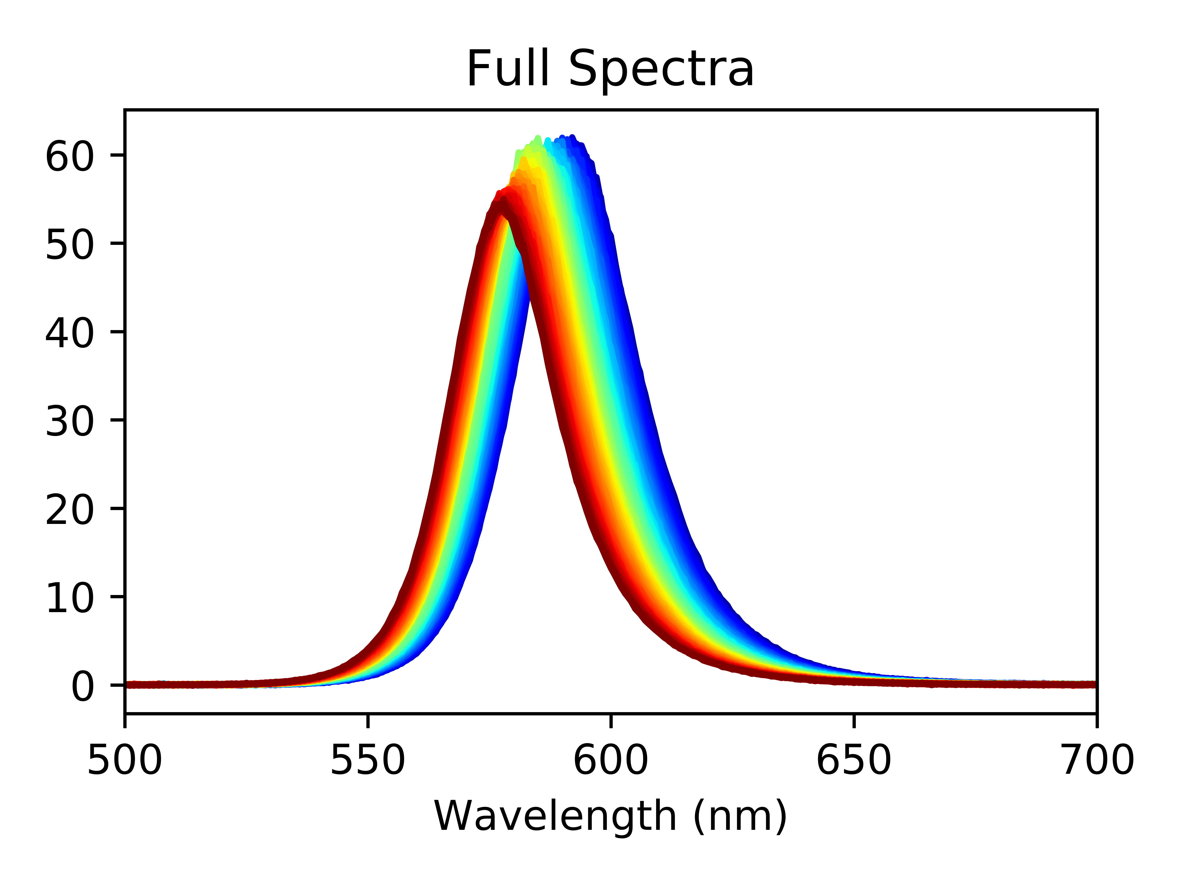
Where the colormap serves as a great way to visualize how far along in the experiment we are; in this case, blue at the start and red at the end. At this point, you can use your data to make a publication quality figure visualizing changes in your spectra over time. You can even select just the scans you want to plot, or zoom in on specific region of the spectra.
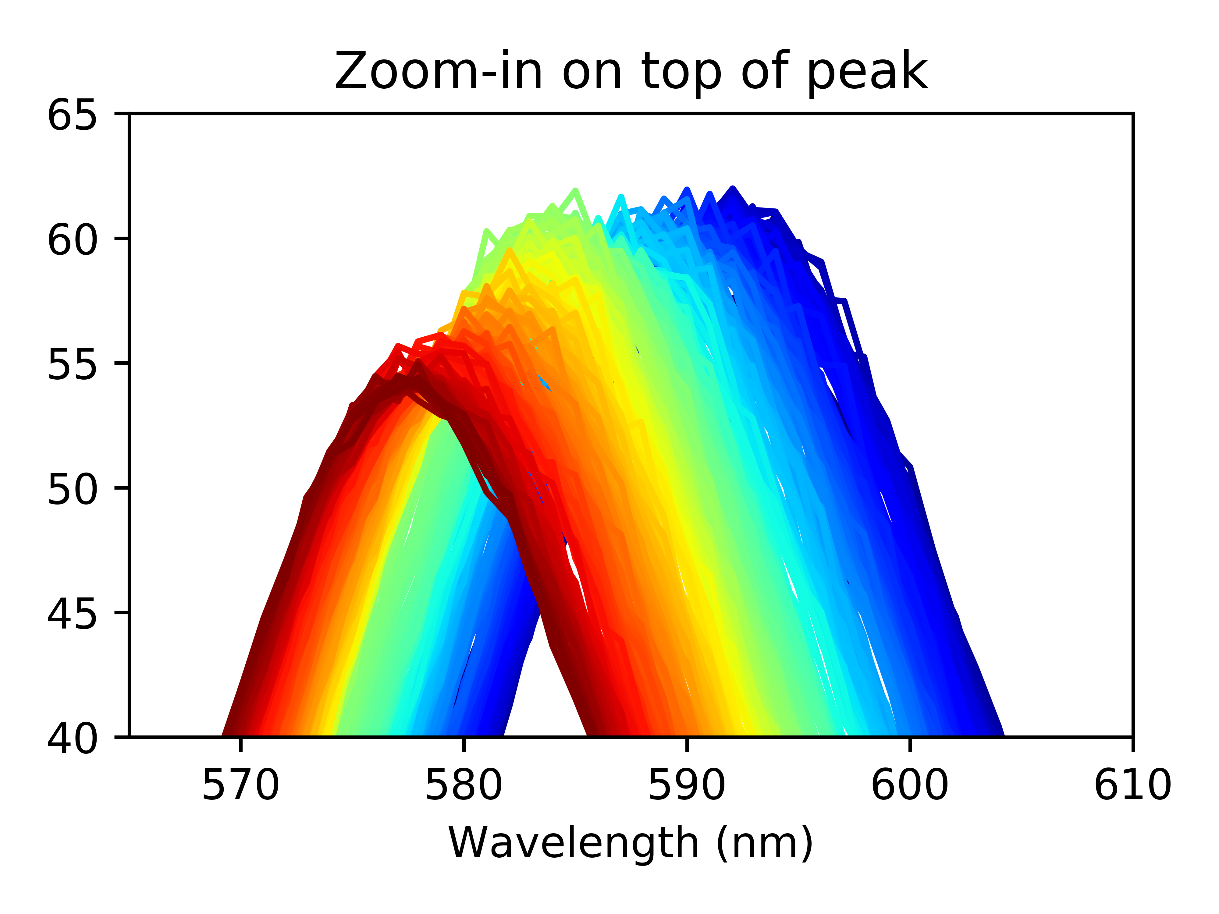
Zooming in on the top of the peaks, we can see a few things off the bat: the peak height decreases as the experiment progesses and the peak center shifts towards lower wavelengths.
Now that our data is clean, we see that it makes sense to fit each peak to a single gaussian curve such that we can extract information about changes to the peak height, center, and width over the course of the reaction.
I have gone into detail about how to fit curves to the various lineshapes (gaussian, lorentzian, voigt) here, which it may be helpful to read and then come back to this section. In short, we need to define an arbitrary gaussian function which we will use to fit each scan of the data, and then iterate over the df observations, fitting each to the single gaussian. We will go one step further, and store each fit to a pre-initialized ndarray, so that we can easily get these values back and work with them.
Once we have the fitting data in ndarry form, we want to convert it to a dataframe so that it's easier to visualize the raw data and clean it up. To do this, we need to create an index column, which in most cases of this type of data will be list or array of times that each scan was collected. The scans in this dataset were collected every 30 seconds, so I will create an array where the elements increase in 0.5 increments, such that our units will be minutes. We then just horizontally stack the index array and our fitting parameter array next to each other, and convert to a dataframe using panda's Dataframe function.
After re-assigning the index and re-labeling the observations, we have a pretty good looking dataframe to work with.
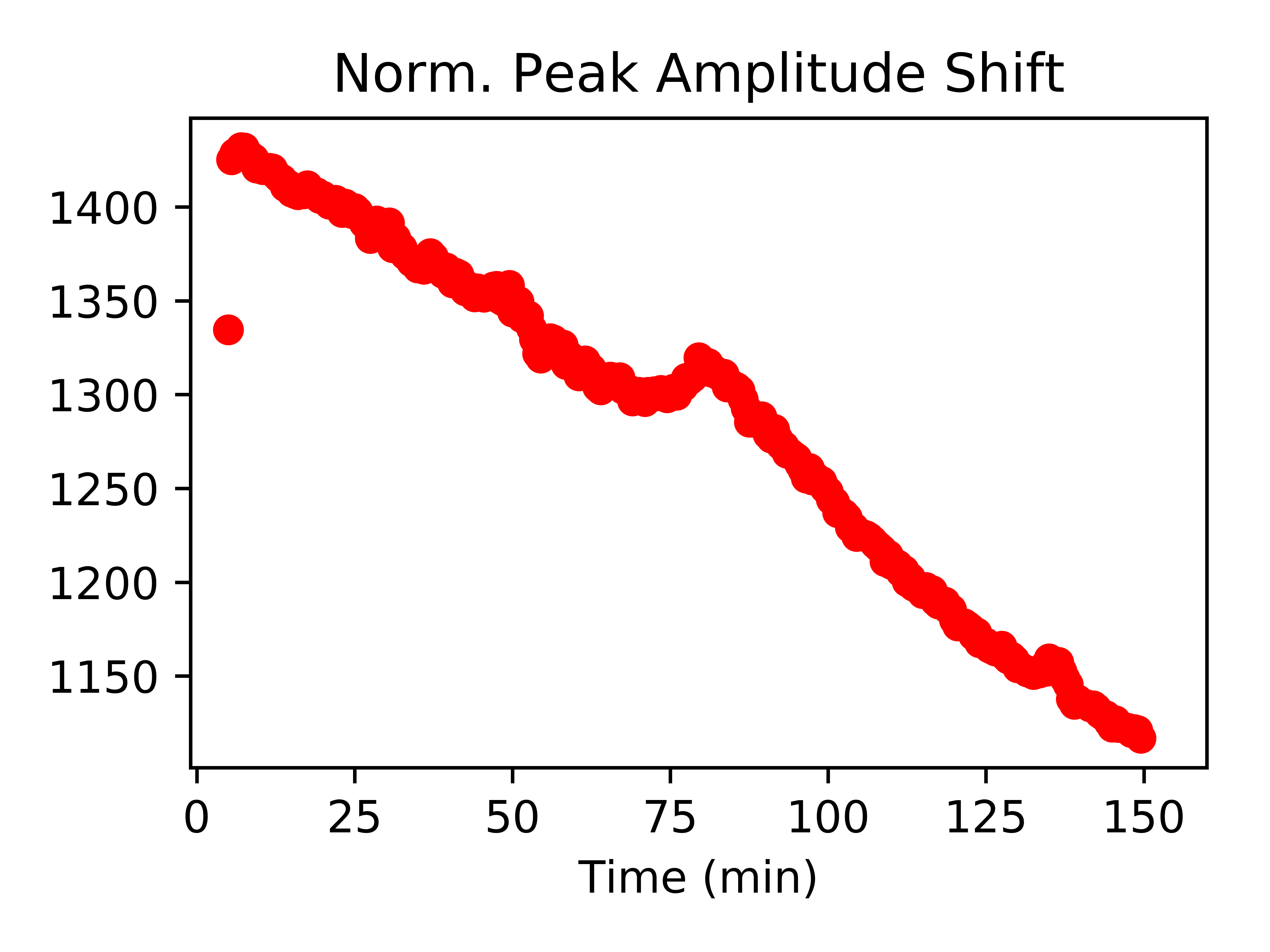
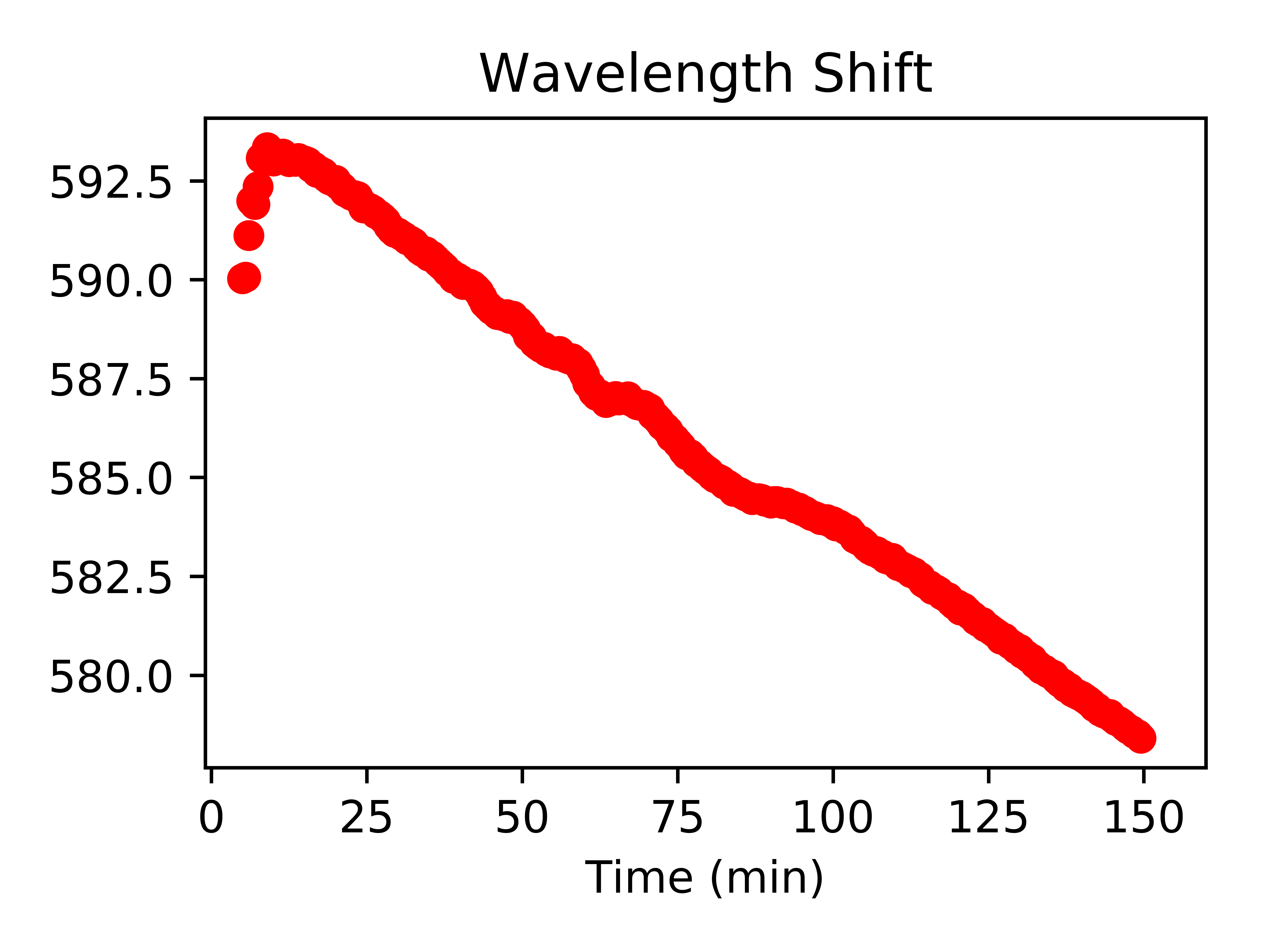
This fitting information tells us so much about our system which underwent this experiment. It is often helpful or necessary to visualize changes to the fitting parameters over time, and fit these curves to various trends, i.e. linear, mono-, or multi-exponential.
Just as with our experimental data dataframe, we can plot the fitting parameters individually using single lines:
fitData_df['Norm. Peak Amplitude'].plot(legend=False,style=["ro"],title="Norm. Peak Amplitude Shift",xlim=(-1,160))
fitData_df['Wavelength (nm)'].plot(legend=False,style=["ro"],title="Wavelength Shift",xlim=(-1,160))
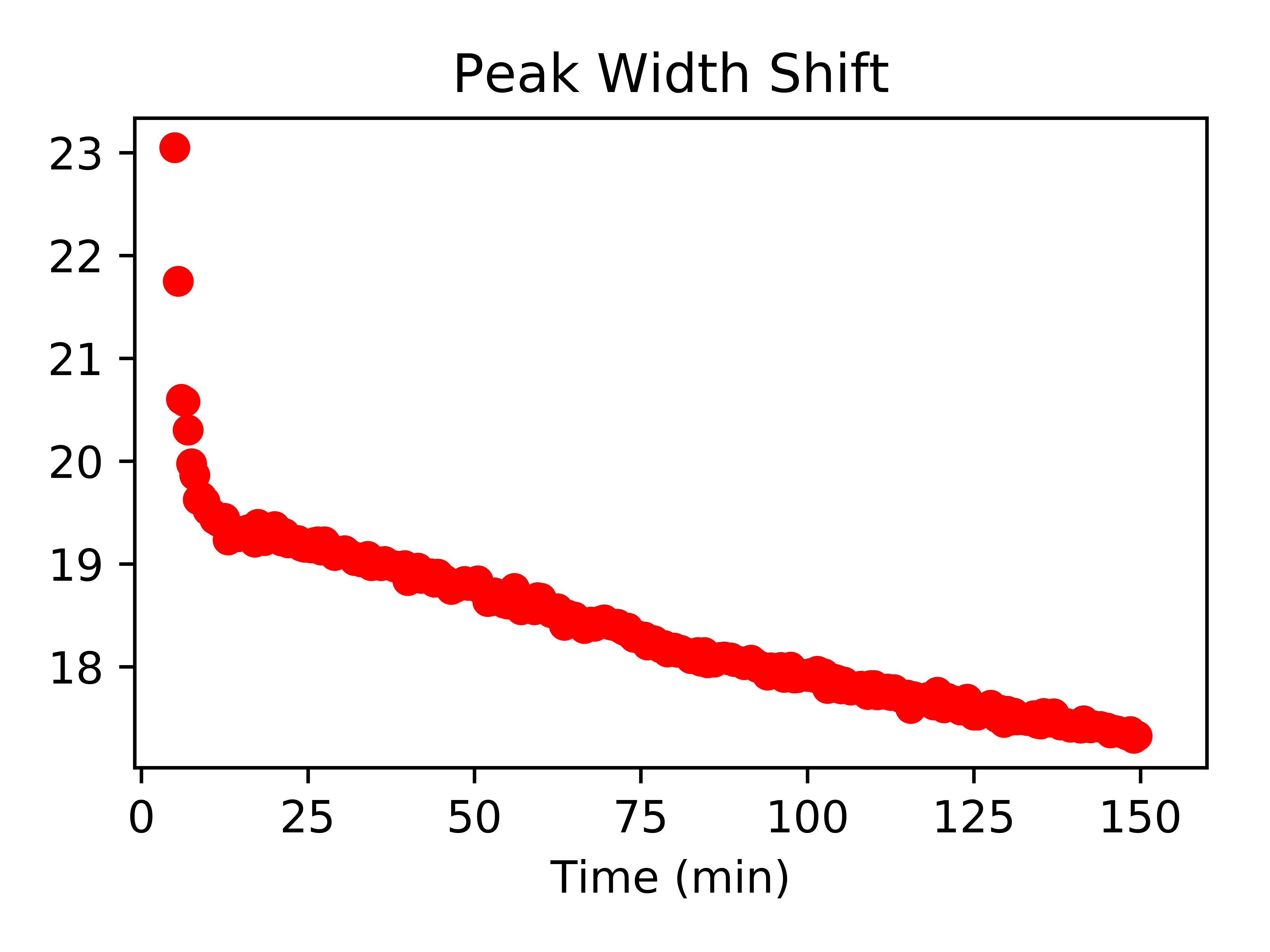
fitData_df['FWHM (nm)'].plot(legend=False,style=["ro"],title="Peak Width Shift",xlim=(-1,160))
To fit these curves to trendlines, reference my previous post on trendline fitting. You can extract information such as reaction rates via this method.
Often it is helpful to save dataframes (or ndarrays) as a file which you can use in other notebooks or scripts, or send to another user to work with your clean data. Depending on what you need, you can save the dataframe as a CSV file, or something called a pickle.
Saving as a pickle just takes your dataframe and saves it as an object identical to what you have. This is helpful for if you know you will be working with this data in python again. If instead you don't care about maintaining your indexing, you can save the data as a CSV file.
All thoughts and opinions are my own and do not reflect those of my institution.