
As a scientist, one of the most powerful python skills you can develop is curve and peak fitting. Whether you need to find the slope of a linear-behaving data set, extract rates through fitting your exponentially decaying data to mono- or multi-exponential trends, or deconvolute spectral peaks to find their centers, intensities, and widths, python allows you to easily do so, and then generate a beautiful plot of your results.
In this series of blog posts, I will show you: (1) how to fit curves, with both linear and exponential examples and extract the fitting parameters with errors, and (2) how to fit a single and overlapping peaks in a spectra. These basic fitting skills are extremely powerful and will allow you to extract the most information out of your data.
I have added the notebook I used to create this blog post, 181113_CurveFitting, to my GitHub repository which can be found here. This post was designed for the reader to follow along in the notebook, and thus this post will be explaining what each cell does/means instead of telling you what to type for each cell. If you don’t know how to open an interactive python notebook, please refer to my previous post.
We will be using the numpy and matplotlib libraries which you should already have installed if you have followed along with my python tutorial, however we will need to install a new package, Scipy. This library is a useful library for scientific python programming, with functions to help you Fourier transform data, fit curves and peaks, integrate of curves, and much more. You can simply install this from the command line like we did for numpy before, with pip install scipy.
One of the most fundamental ways to extract information about a system is to vary a single parameter and measure its effect on another. This data can then be interpreted by plotting is independent variable (the unchanging parameter) on the x-axis, and the dependent variable (the variable parameter) on the y-axis. Usually, we know or can find out the empirical, or expected, relationship between the two variables which is an equation. This relationship is most commonly linear or exponential in form, and thus we will work on fitting both types of relationships.
For the sake of example, I have created some fake data for each type of fitting. To do this, I do something like the following:
x_array = np.linspace(1,10,10)
y_array = np.linspace(5,200,10)
y_noise = 30*(np.random.ranf(10))
y_array += y_noise
I use a function from numpy called linspace which takes in the first number in a range of data (1), the last number in the range (10), and then how many data points you want between the two range end-values (10). I assign this to x_array, which will be our x-axis data. What this does is creates a list of ten linearly-spaced numbers between 1 and 10: [1,2,3,4,5,6,7,8,9,10]. You can picture this as a column of data in an excel spreadsheet.
Next, I create a list of y-axis data in a similar fashion and assign it to y_array. This will be our y-axis data.
I want to add some noise (y_noise) to this data so it isn’t a perfect line. To do this, I use a function from numpy called random.ranf which takes in 1 number (10) which is the number of random numbers you want, and it returns a list of this number of random “floats” (which means they are numbers with decimals) between 0.0 and 1.0. I then multiply these numbers by 30 so they aren’t so small, and then add the noise to the y_array.
Now we have some linear-behaving data that we can work with:
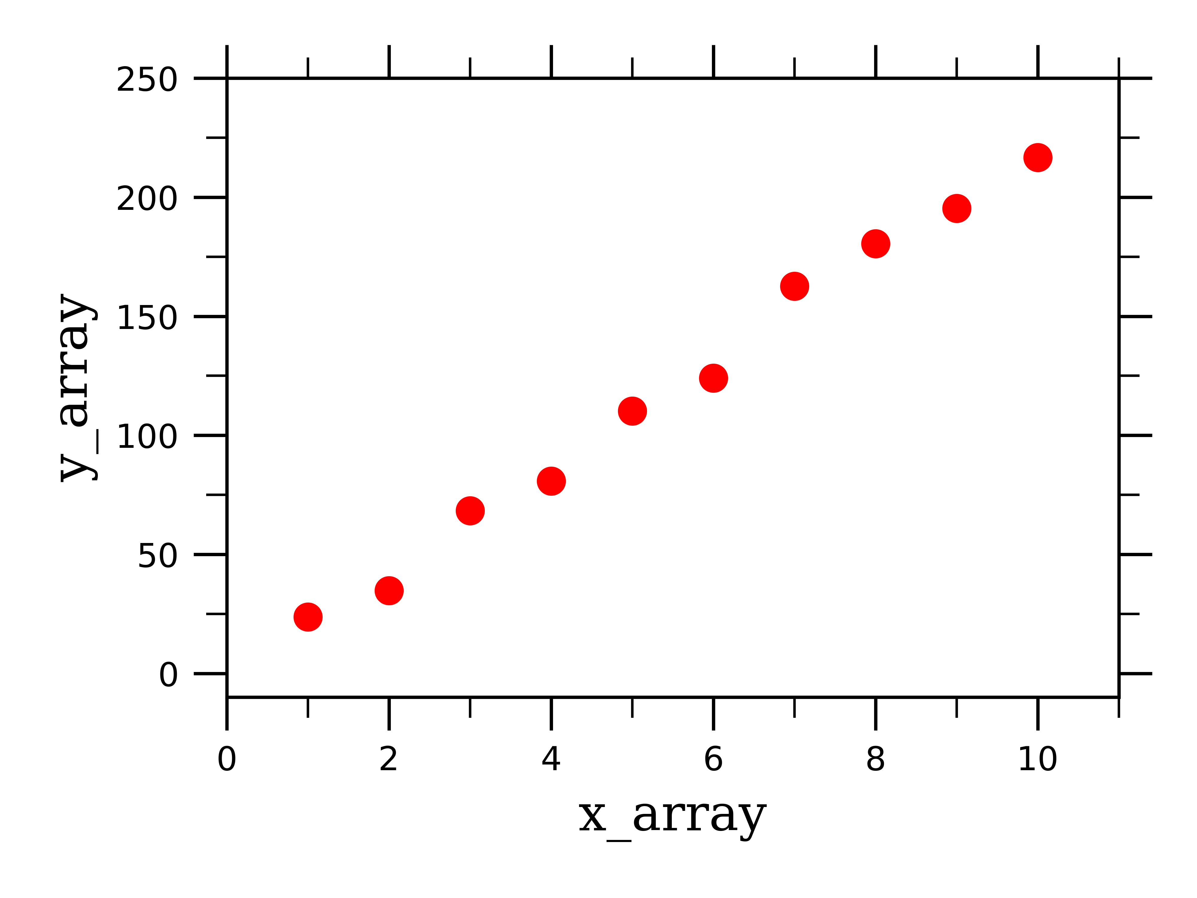
To fit this data to a linear curve, we first need to define a function which will return a linear curve:
def linear(x, m, b):
    return m*x + b
We will then feed this function into a scipy function:
popt_linear, pcov_linear = scipy.optimize.curve_fit(linear, x_array, y_array, p0=[((75-25)/(44-2)), 0])
The scipy function “scipy.optimize.curve_fit” takes in the type of curve you want to fit the data to (linear), the x-axis data (x_array), the y-axis data (y_array), and guess parameters (p0). The function then returns two pieces of information: popt_linear and pcov_linear, which contain the actual fitting parameters (popt_linear), and the covariance of the fitting parameters(pcov_linear).
We can then solve for the error in the fitting parameters, and print the fitting parameters:
perr_linear = np.sqrt(np.diag(pcov_linear))
print "slope = %0.2f (+/-) %0.2f" % (popt_linear[0], perr_linear[0])
print "y-intercept = %0.2f (+/-) %0.2f" %(popt_linear[1], perr_linear[1])
This returns the following:
slope = 22.31 (+/-) 0.67
y-intercept = -3.00 (+/-) 4.18
Finally, we can plot the raw linear data along with the best-fit linear curve:
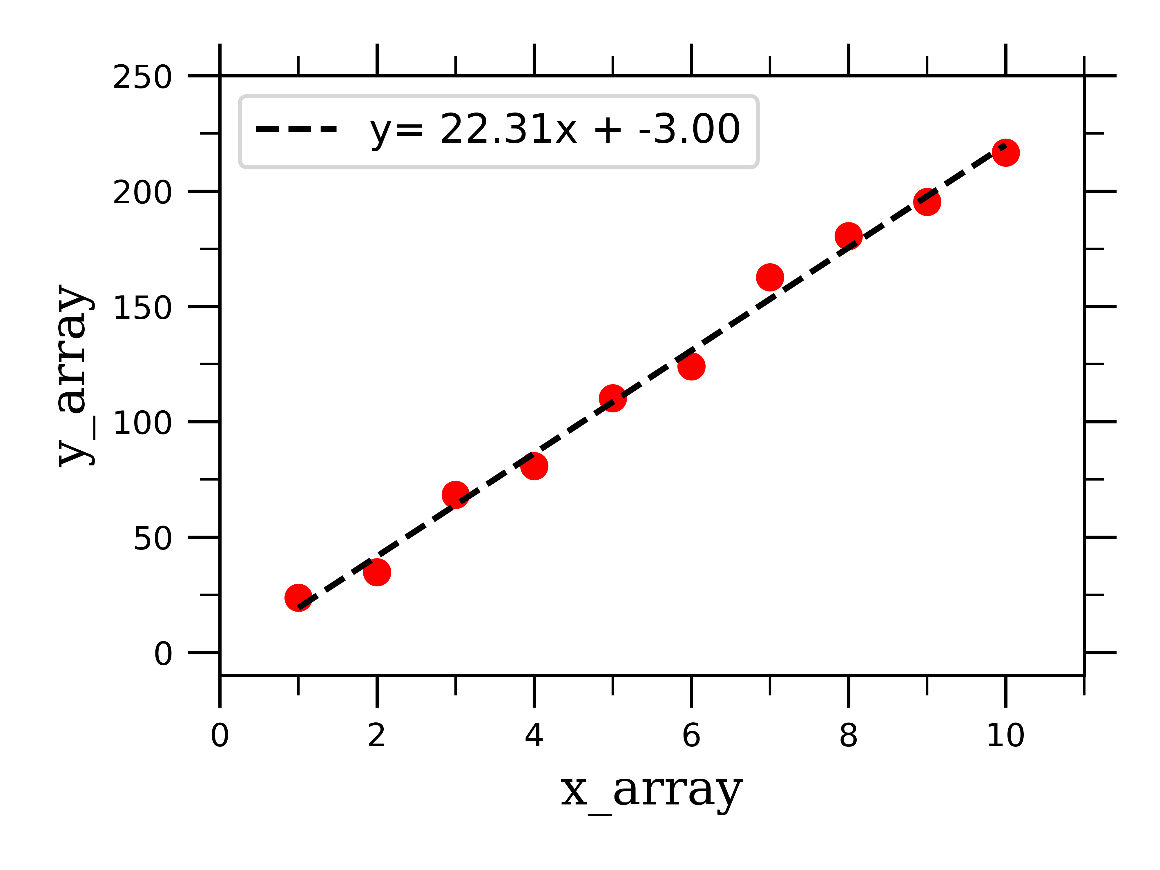
You are now equipped to fit linearly-behaving data! Let’s now work on fitting exponential curves, which will be solved very similarly.
Exponential growth and/or decay curves come in many different flavors. Most importantly, things can decay/grow mono- or multi- exponentially, depending on what is effecting their decay/growth behavior. I will show you how to fit both mono- and bi-exponentially decaying data, and from these examples you should be able to work out extensions of this fitting to other data systems.
As previously, we need to construct some fake exponentially-behaving data to work with where y_array is exponentially rather than linearly dependent on x_array, and looks something like this:
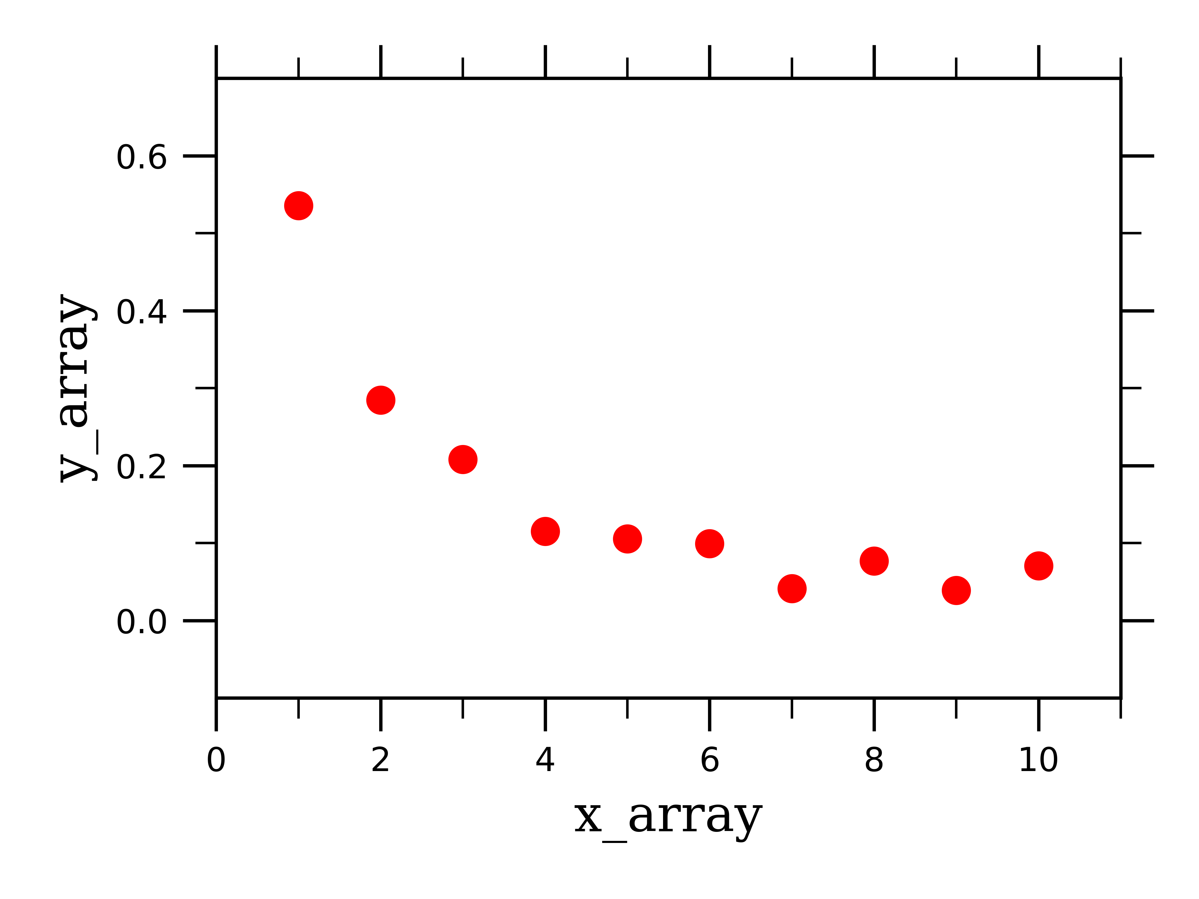
We next need to define a new function to fit exponential data rather than linear:
def exponential(x, a, k, b):
    return a*np.exp(x*k) + b
Just as before, we need to feed this function into a scipy function:
popt_exponential, pcov_exponential = scipy.optimize.curve_fit(exponential, x_array, y_array_exp, p0=[1,-0.5, 1])
And again, just like with the linear data, this returns the fitting parameters and their covariance.
Solving for and printing the error of this fitting parameters, we get:
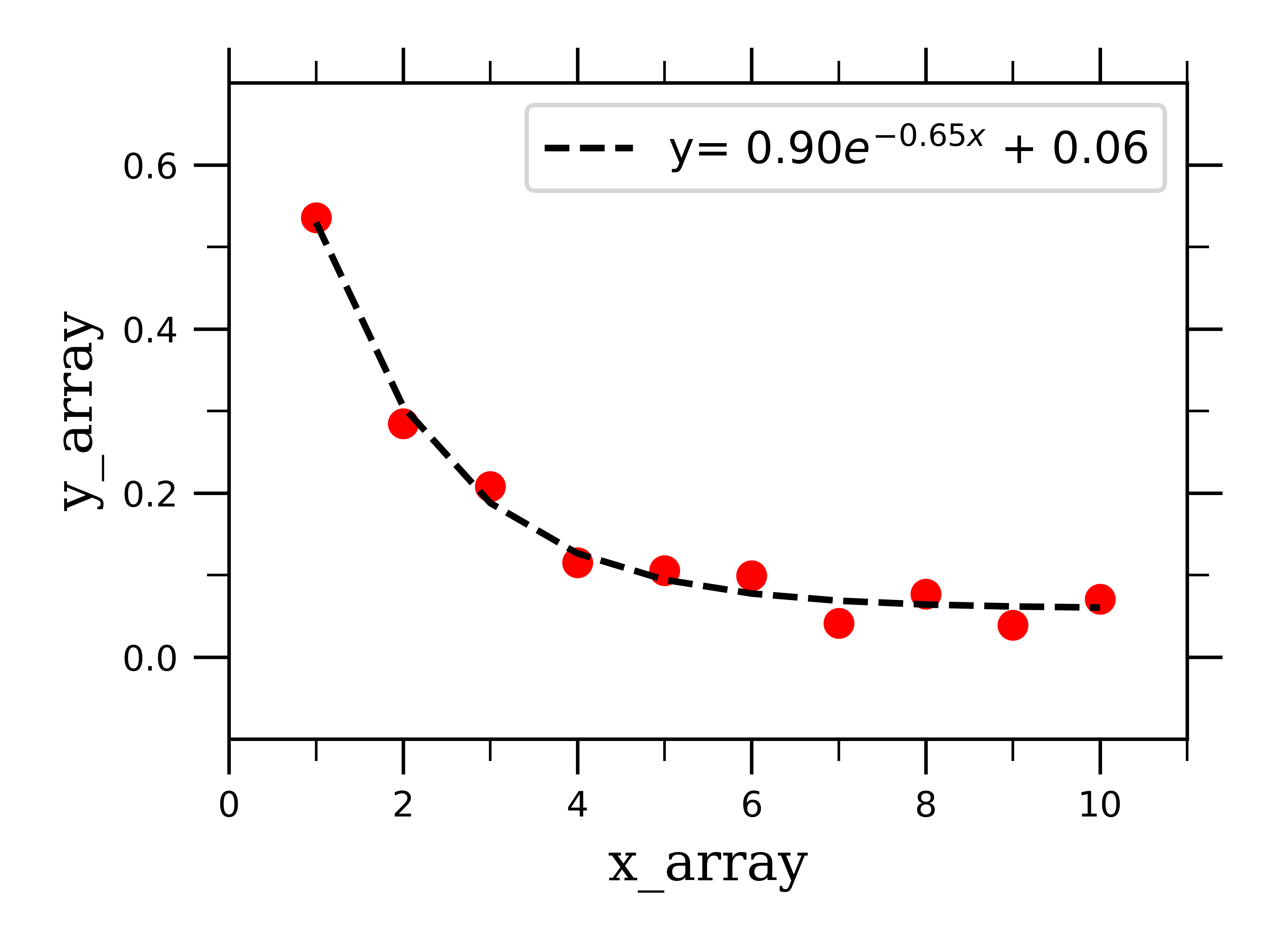
pre-exponential factor = 0.90 (+/-) 0.08
rate constant = -0.65 (+/-) 0.07
Plotting the raw linear data along with the best-fit exponential curve:
We can similarly fit bi-exponentially decaying data by defining a fitting function which depends on two exponential terms:
def _2exponential(x, a, k1, b, k2, c):
    return a*np.exp(x*k1) + b*np.exp(x*k2) + c
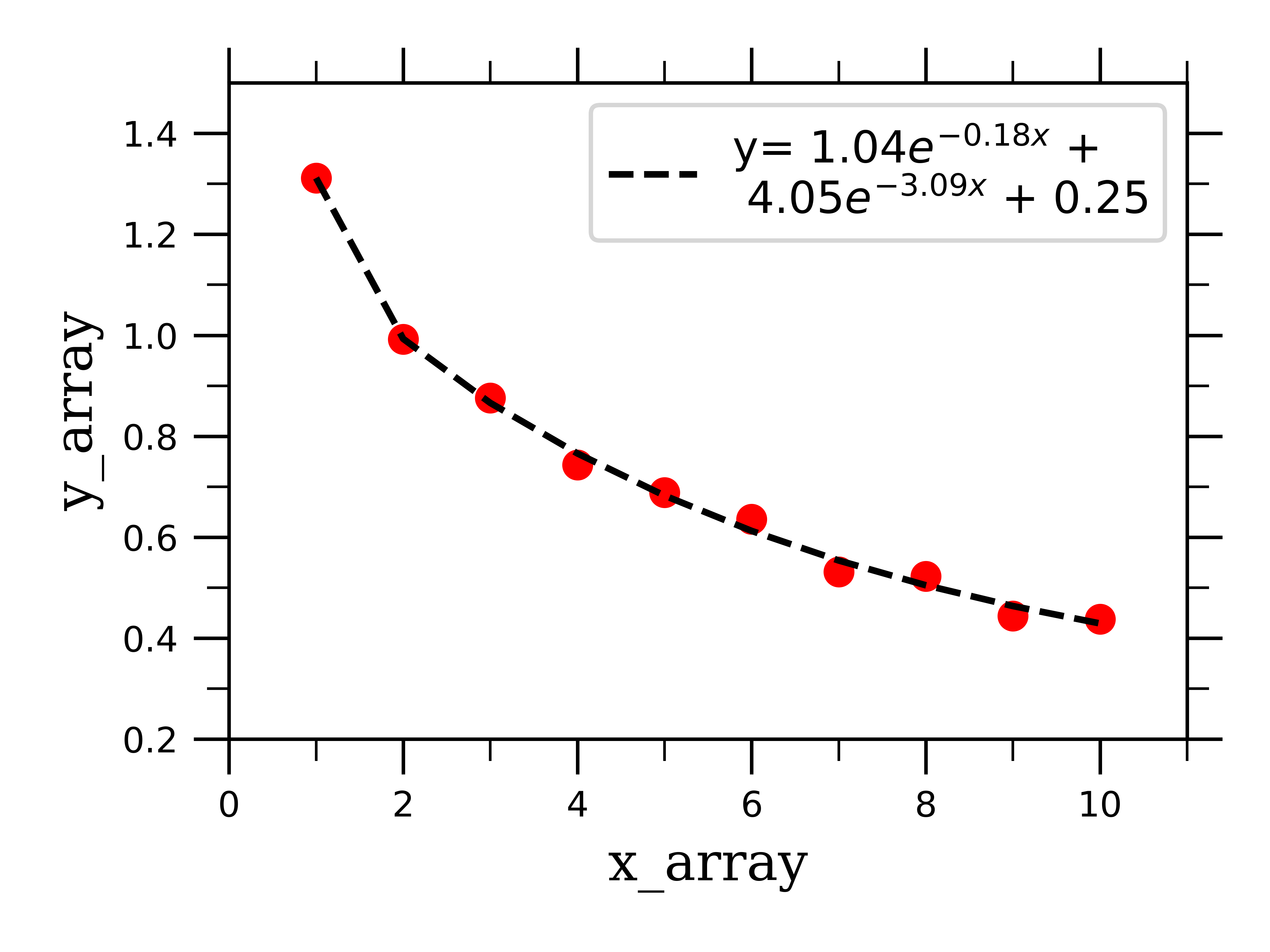
If we feed this into the scipy function along with some fake bi-exponentially decaying data, we can successfully fit the data to two exponentials, and extract the fitting parameters for both:
pre-exponential factor 1 = 1.04 (+/-) 0.08
rate constant 1 = -0.18 (+/-) 0.06
pre-exponential factor 2 = 4.05 (+/-) 0.01
rate constant 2 = -3.09 (+/-) 5.99
As you can see, the process of fitting different types of data is very similar, and as you can imagine can be extended to fitting whatever type of curve you would like. Stay tuned for the next post in this series where I will be extending this fitting method to deconvolute over-lapping peaks in spectra.
All thoughts and opinions are my own and do not reflect those of my institution.