
The abundance of software available to help you fit peaks inadvertently complicate the process by burying the relatively simple mathematical fitting functions under layers of GUI features. As I hope you have seen in Part I of this series, in can be quite empowering to be able to fit all of your data from scratch instead of using peak-fitting software in this case. With this post, I want to continue to inspire you to ditch the GUIs and use python to work up your data by showing you how to fit spectral peaks with line-shapes and extract an abundance of information to aid in your analysis.
I have added the notebook I used to create this blog post, 181119_PeakFitting, to my GitHub repository which can be found here. As was the previous post, this post was designed for the reader to follow along in the notebook, and thus this post will be explaining what each cell does/means instead of telling you what to type for each cell.
First we will focus on fitting single and multiple gaussian curves. First I created some fake gaussian data to work with (see notebook and previous post):
As you can see, this generates a single peak with a gaussian lineshape, with a specific center, amplitude, and width. We then want to fit this peak to a single gaussian curve so that we can extract these three parameters. To do so, just like with linear or exponential curves, we define a fitting function which we will feed into a scipy function to fit the fake data:
def _1gaussian(x, amp1,cen1,sigma1):
    return amp1*(1/(sigma1*(np.sqrt(2*np.pi))))*(np.exp((-1.0/2.0)*(((x_array-cen1)/sigma1)**2)))
I constructed this fitting function by using the basic equation of a gaussian distribution. We then feed this function into a scipy function, along with our x- and y-axis data, and our guesses for the function fitting parameters (for which I use the center, amplitude, and sigma values which I used to create the fake data):
popt_gauss, pcov_gauss = scipy.optimize.curve_fit(_1gaussian, x_array, y_array_gauss, p0=[amp1, cen1, sigma1])
perr_gauss = np.sqrt(np.diag(pcov_gauss))
We can then print out the three fitting parameters with their respective errors:
amplitude = 122.80 (+/-) 3.00
center = 49.90 (+/-) 0.33
sigma = 11.78 (+/-) 0.33
And then plot our data along with the fit:
This fit does a pretty good job at fitting the fake gaussian data. Now that we can successfully fit a well-resolved single gaussian, peak, lets work on the more complicated case where we have several overlapping peaks which need to be convoluted from one another.
It is extremely helpful to be able to fit several overlapping peaks, because usually spectral features are not well-resolved from one another, and even a portion of the tail of a gaussian curve can skew the fit of another curve if they are overlapping. We will consider a strongly overlapping region of data:
In the fake data above, you can see that there are two gaussian peaks whose features (i.e. peak center and width) can’t be distinguished from one another. In my research, I come across this case often when I am looking at Fluorescence spectra of species who emit at similar wavelength, and I am interested in the relative areas under the two curves; thus I need to deconvolute (or separate) these two curves from one another.
Just like with the bi-exponential fit we previously investigated, in order to fit overlapping gaussian peaks, we need to define a function for the sum of two gaussians:
def _2gaussian(x, amp1,cen1,sigma1, amp2,cen2,sigma2):
    return amp1*(1/(sigma1*(np.sqrt(2*np.pi))))*(np.exp((-1.0/2.0)*(((x_array-cen1)/sigma1)**2))) + \
            amp2*(1/(sigma2*(np.sqrt(2*np.pi))))*(np.exp((-1.0/2.0)*(((x_array-cen2)/sigma2)**2)))
You can see that the only difference between _1gaussian and _2gaussian is that the later is a sum of two gaussian functions and fits six parameters rather than three in the former.
Feeding this into scipy works the same way:
popt_2gauss, pcov_2gauss = scipy.optimize.curve_fit(_2gaussian, x_array, y_array_2gauss, p0=[amp1, cen1, sigma1, amp2, cen2, sigma2])
perr_2gauss = np.sqrt(np.diag(pcov_2gauss))
pars_1 = popt_2gauss[0:3]
pars_2 = popt_2gauss[3:6]
gauss_peak_1 = _1gaussian(x_array, *pars_1)
gauss_peak_2 = _1gaussian(x_array, *pars_2)
However, I added a few more lines of code to define pars_1, pars_2, and gauss_peak_1, gauss_peak_2. The pars variables are arrays which hold just the fitting parameters for the first and second peaks respectively. We want to define these variables because we can then feed them into our _1gaussian function to construct data for the stand-alone peaks.
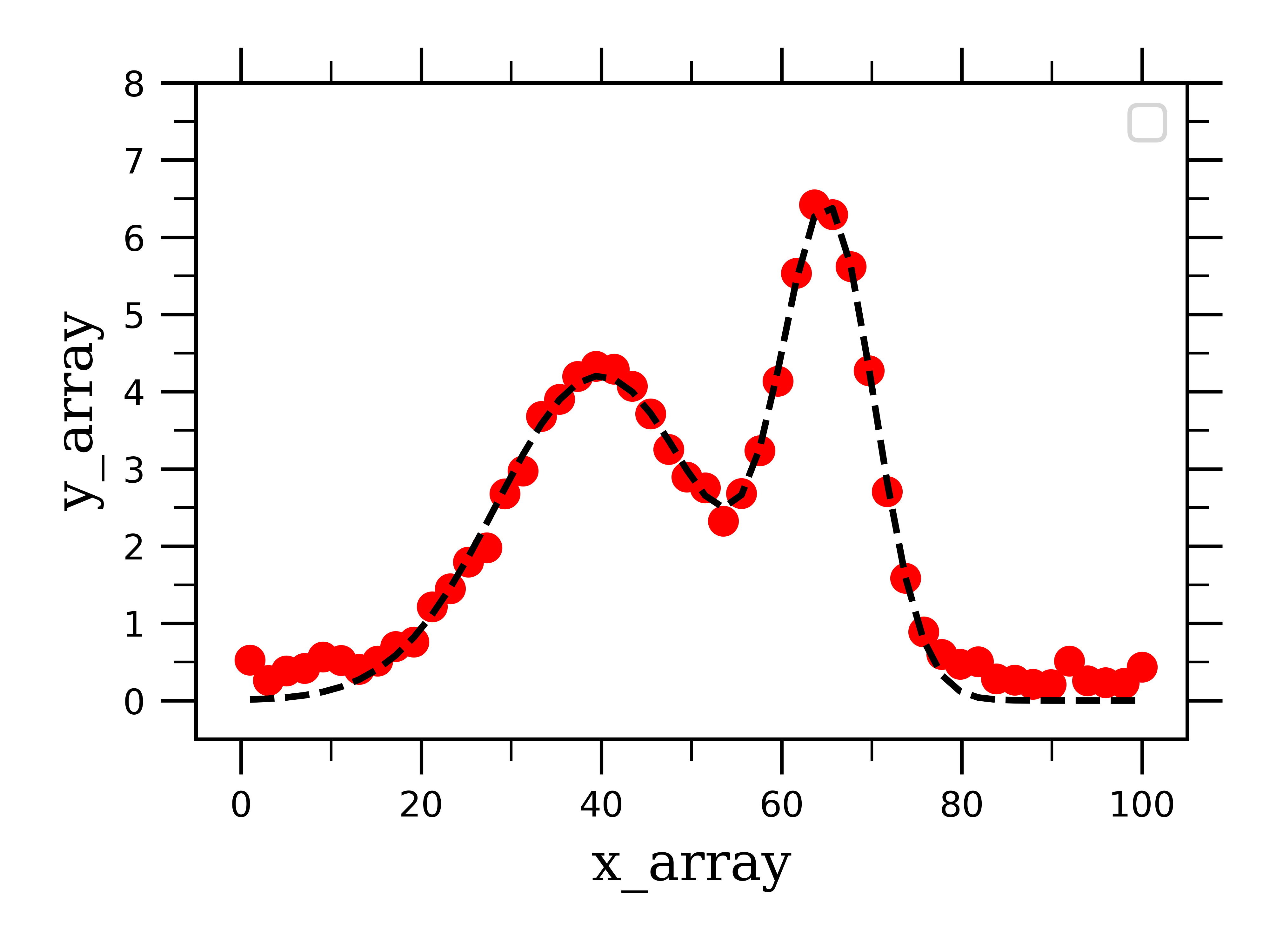
If we plot our fake two-gaussian data and the _2gaussian fit, we see that the data (red dots) is traced nicely by the fit (dashed black line).
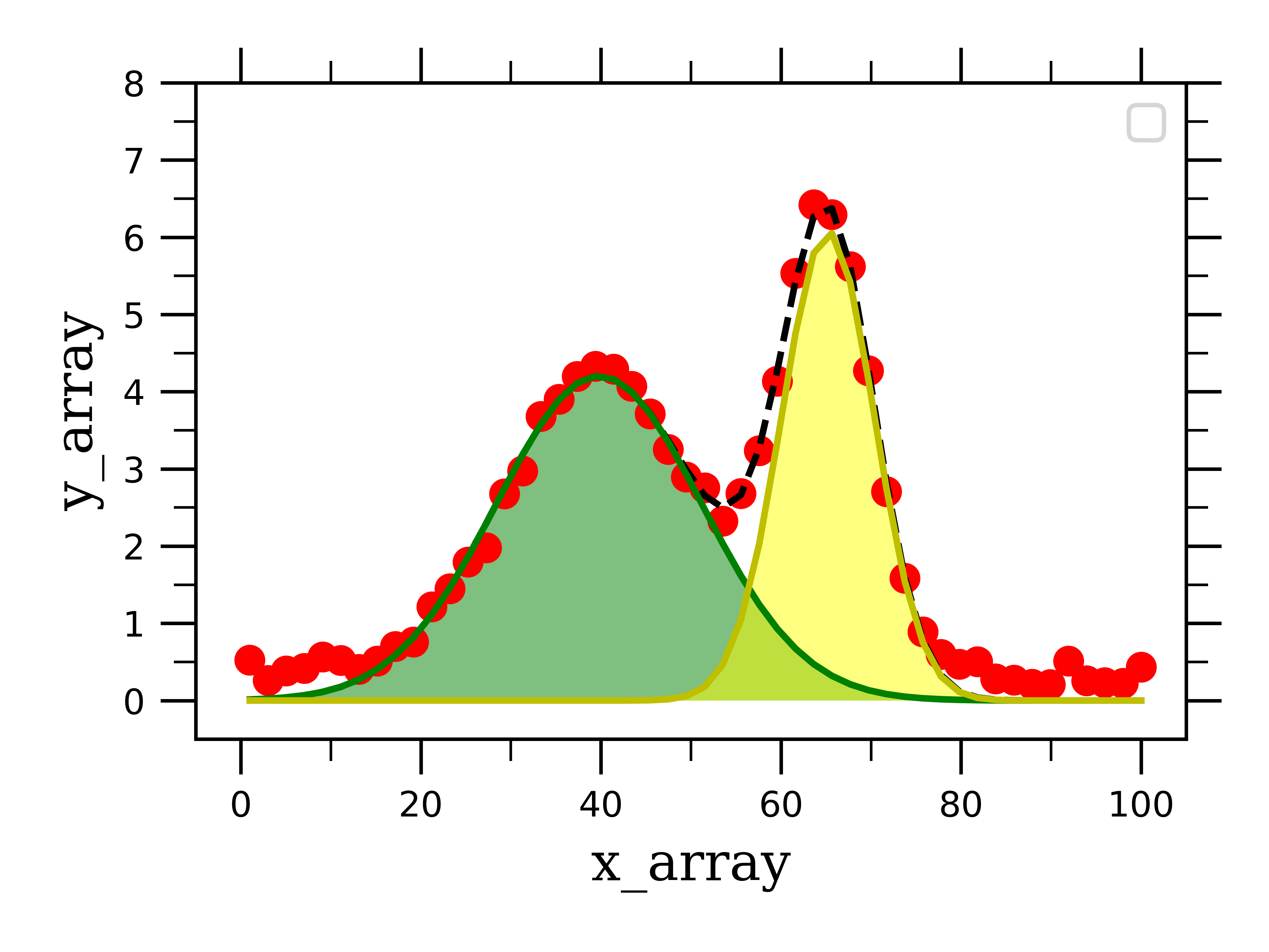
However, we want to be able to see the peaks on their own after they have been separated from one another. This is where the gauss_peak_1 and _2 variables come into play.
If we add the following lines of code into our plotting cell, we can plot the two peaks on their own:
ax1.plot(x_array, gauss_peak_1, "g")
ax1.fill_between(x_array, gauss_peak_1.min(), gauss_peak_1, facecolor="green", alpha=0.5)

ax1.plot(x_array, gauss_peak_2, "y")
ax1.fill_between(x_array, gauss_peak_2.min(), gauss_peak_2, facecolor="yellow", alpha=0.5)
This employs a function called “fill_between” from the matplotlib library. I like using this function because it allows us to see that area that each peak occupies under the total curve:
We can then print the fitting parameters of the two curves, as well as the area under the curves to extract all the desired information to analyze our system:
-------------Peak 1-------------
amplitude = 120.09 (+/-) 3.54
center = 39.80 (+/-) 0.37
sigma = 11.39 (+/-) 0.41
area = 59.42
--------------------------------
-------------Peak 2-------------
amplitude = 78.51 (+/-) 2.73
center = 65.22 (+/-) 0.16
sigma = 5.15 (+/-) 0.16
area = 38.86
--------------------------------
A common (an important) way to visualize your data is to plot the residual of your data along with the fit. The residual is just what it sounds like; the portion of the data that is left over, or resides, after you fit the data. In other words, the portion of the data that was not fit. To find the residual, we can do the following:
residual_2gauss = y_array_2gauss - (_2gaussian(x_array, *popt_2gauss))
Further, we take the y-axis data (y_array_2gauss) and subtract the fit from it (_2gaussian(x_array, *popt_2gauss)), and assign this to residual_2gauss. I like to add this to the figure with the deconvoluted signals as a subplot below the original fit data:
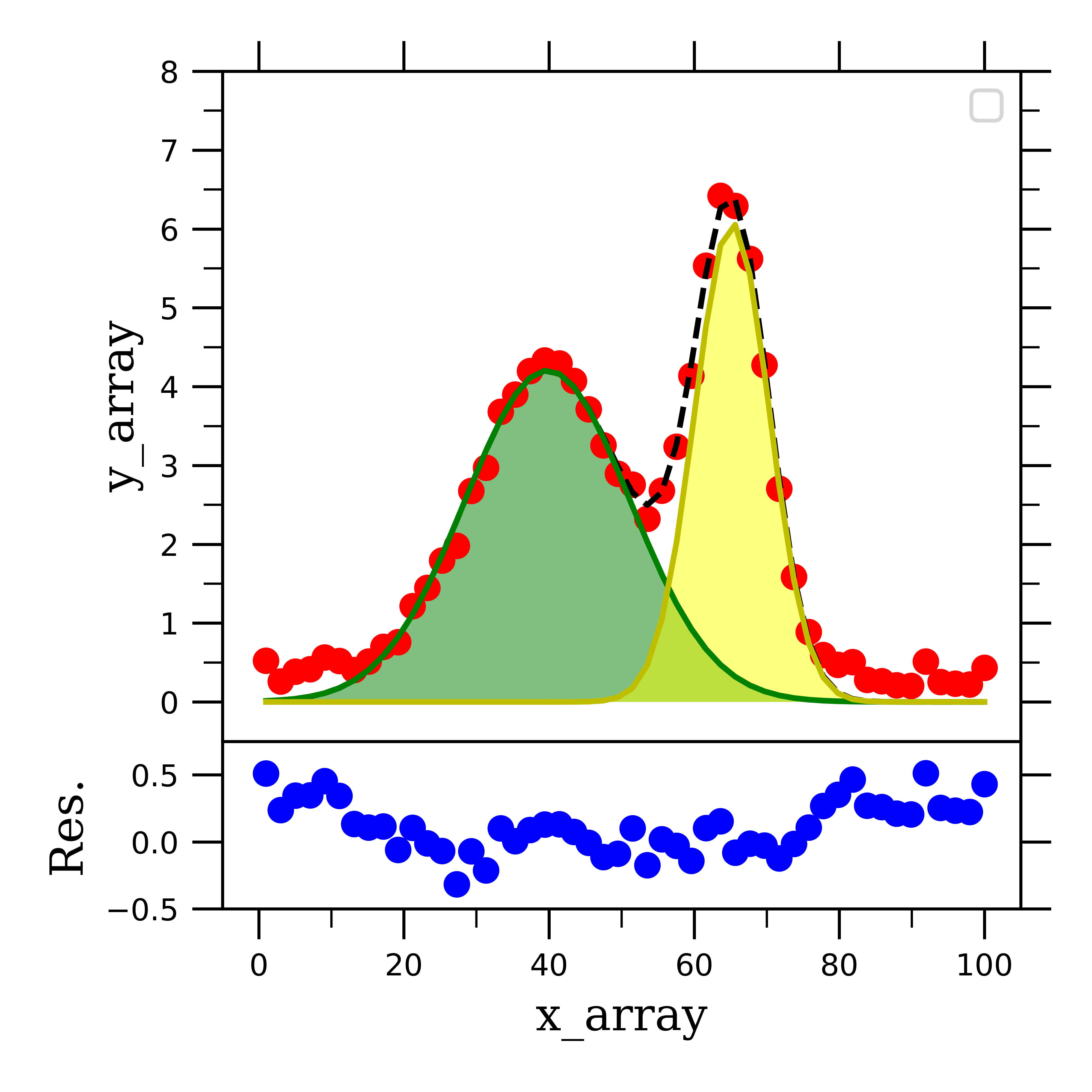
This figure is the complete picture of what deconvoluting two gaussian curves from each other results in. I hope that you can see how you would be able to translate this procedure into fitting more than two curves for more complicated spectra.
Now that we have gaussian lineshapes under our belt, I want to quickly show you how to fit Lorentzian and Voigt lineshape peaks. To do so, I will follow the same exact process, except I will define new fitting functions of the Lorentzian and Voigt type.
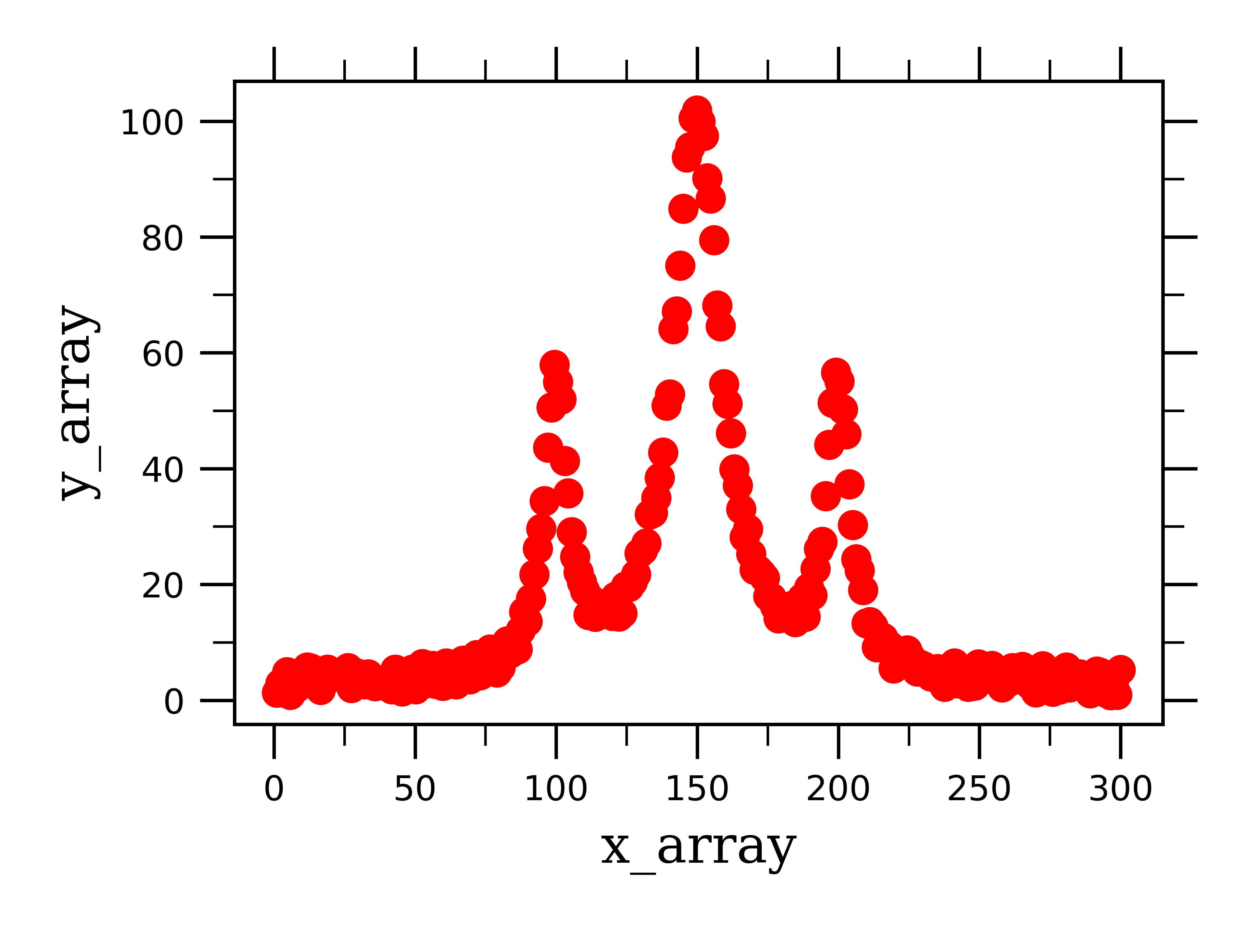
To give you more practice/examples of peak fitting, I will illustrate how to fit Lorentzian peaks with three overlapping peaks. This is an example of the type data that is acquired from NMR spectroscopy, where peaks have a Lorentzian lineshape, and there are often overlapping multiplets of peaks.
The fitting function we use here is for the sum of three Lorentzian functions.
def _3Lorentzian(x, amp1, cen1, wid1, amp2,cen2,wid2, amp3,cen3,wid3):
    return (amp1*wid1**2/((x-cen1)**2+wid1**2)) +\
            (amp2*wid2**2/((x-cen2)**2+wid2**2)) +\
                (amp3*wid3**2/((x-cen3)**2+wid3**2))
When we fit the three-lorentzian data with this function, we can print out the following information about the three peaks:
-------------Peak 1-------------
amplitude = 50.26 (+/-) 1.07
center = 100.11 (+/-) 0.13
width = 5.84 (+/-) 0.18
area = 746.81
--------------------------------
-------------Peak 2-------------
amplitude = 100.45 (+/-) 0.80
center = 150.12 (+/-) 0.08
width = 10.60 (+/-) 0.13
area = 2659.01
--------------------------------
-------------Peak 3-------------
amplitude = 50.81 (+/-) 1.10
center = 200.11 (+/-) 0.12
width = 5.57 (+/-) 0.18
area = 720.14
--------------------------------
If we then solve for the residual and plot our total fitting information, we can see that this fitting function does a pretty good job at fitting the data:
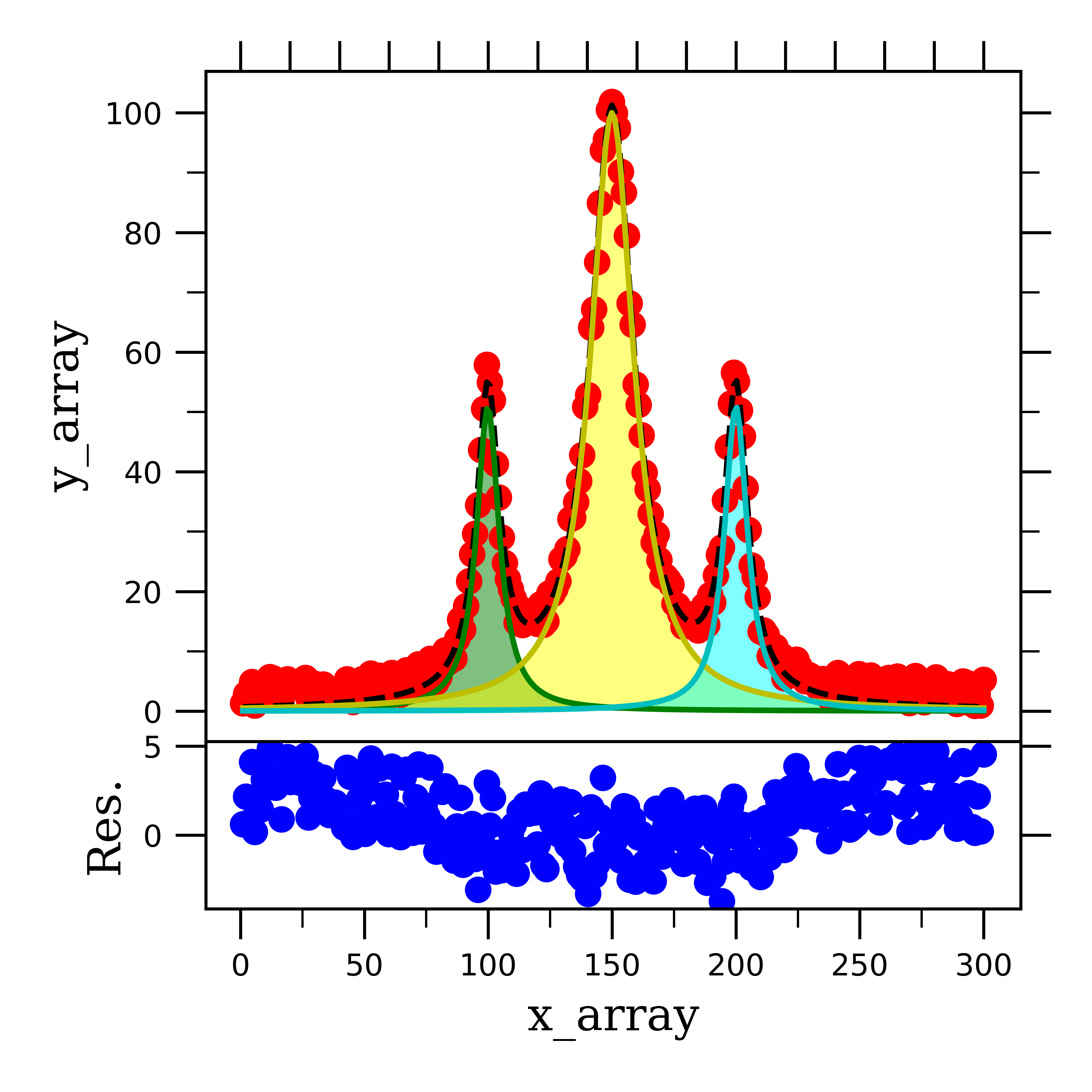
As you can see, fitting Lorentzian lineshape peaks is very similar to gaussian peaks, save the fitting function. Lastly, we will look at how to fit a Voigt lineshape peak.
Not surprisingly, fitting Voigt lineshape peaks follows the same procedure as fitting all other types of data we have looked at so far. In case you didn’t know, Voigt lineshapes are a combination of Lorentzian and Gaussian lineshapes. This kind of peak is common in X-ray diffraction spectroscopy, where we diffract X-ray beams off of solid materials. This can cause the peak to broaden by both Gaussian and Lorentzian mechanisms.
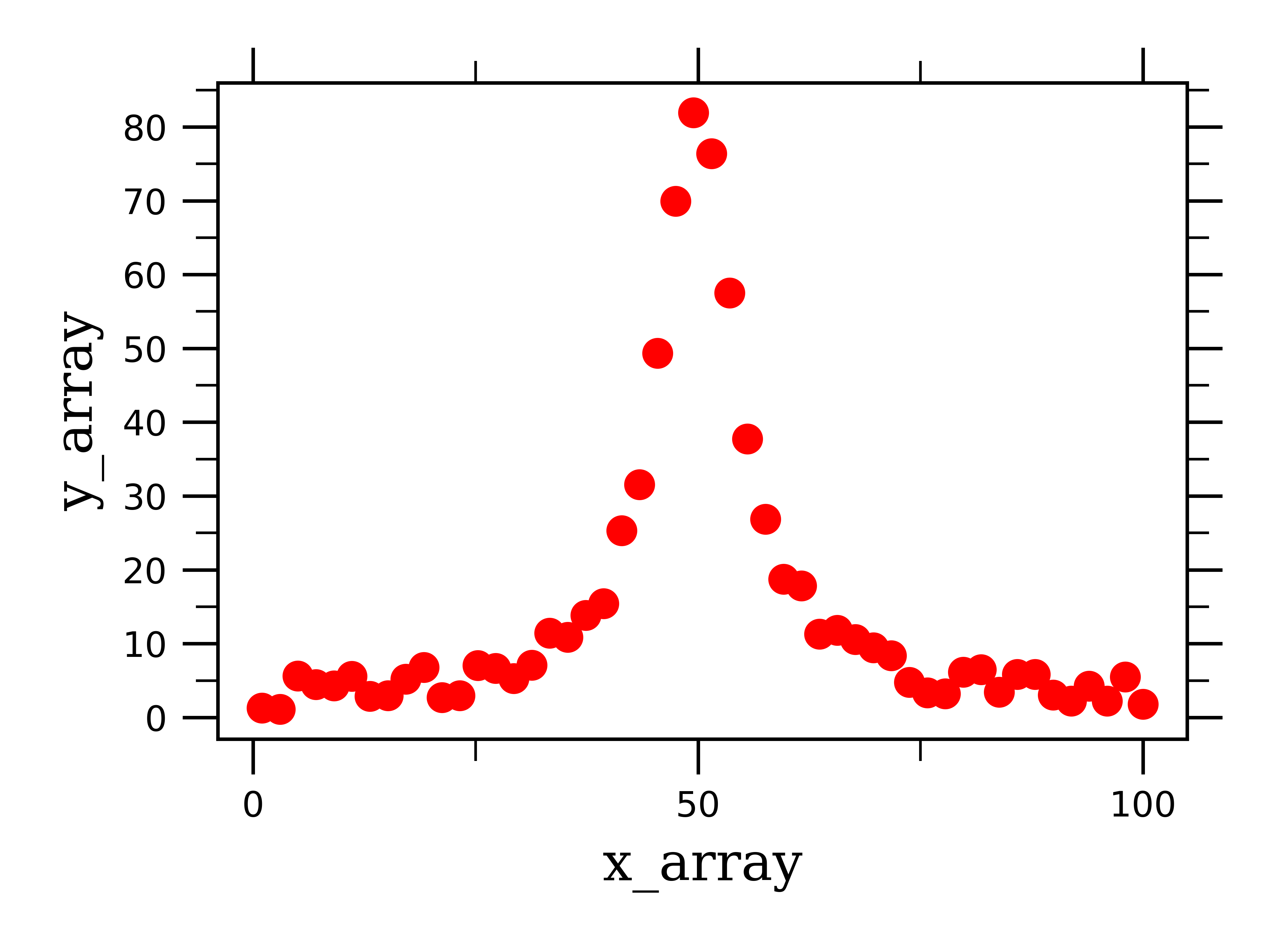
You can see how the peak is more pointed, which is a feature of a Lorentzian peak, whereas as you get closer to the baseline, the peak broadens out, a feature of Gaussian curves (i.e. normal distributions).
The fitting function we use to fit a Voigt lineshape peak is thus a weighted sum of Gaussian and Lorentzian functions:
def _1Voigt(x, ampG1, cenG1, sigmaG1, ampL1, cenL1, widL1):
    return (ampG1*(1/(sigmaG1*(np.sqrt(2*np.pi))))*(np.exp(-((x-cenG1)**2)/((2*sigmaG1)**2)))) +\
              ((ampL1*widL1**2/((x-cenL1)**2+widL1**2)) )
When we feed this into the scipy fitting function, we see, as expected, that this function fits the data quite well:
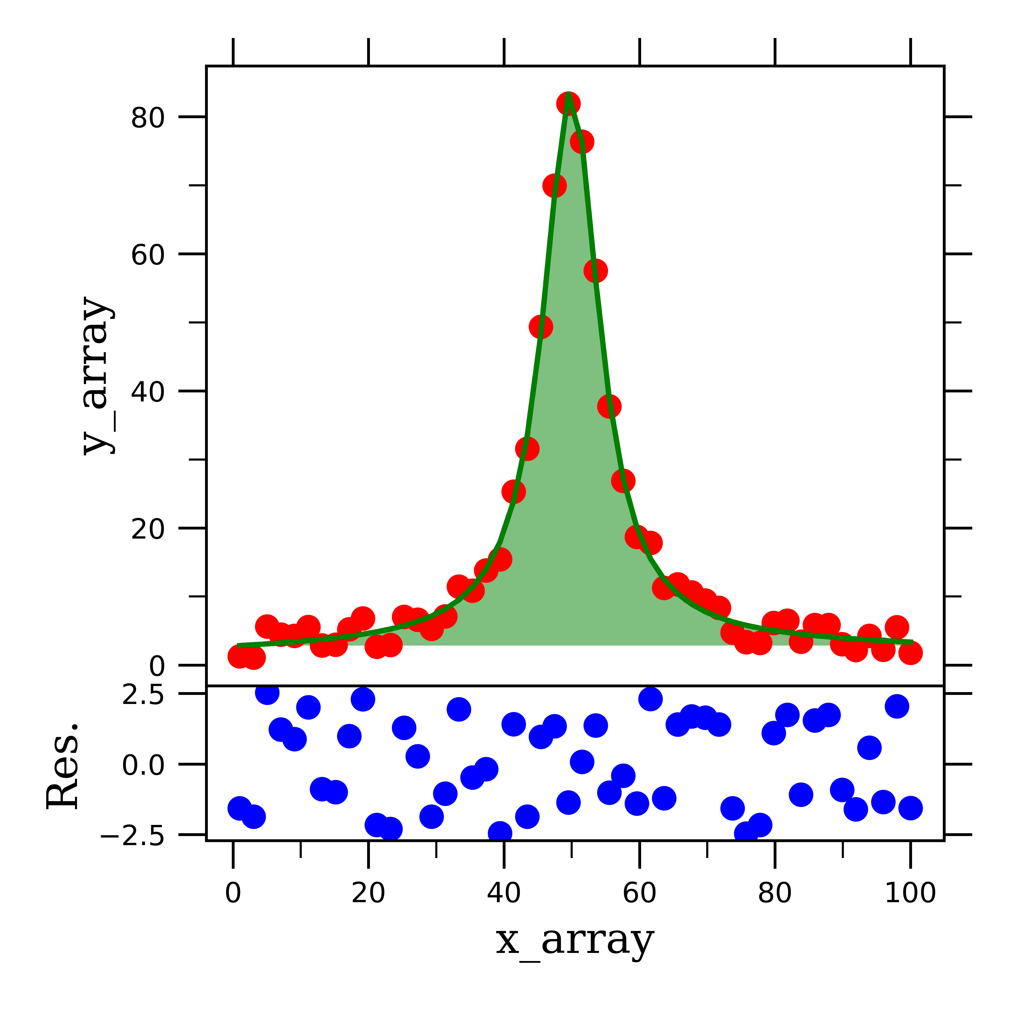
One last thing to point out about this Voigt fitting function, is that because we have Gaussian and Lorentzian weighting parameters (i.e. amplitude), we can use these to analyze how much of the peak broadening is from the respective broadening mechanisms! That’s pretty cool!
gauss. weight = 84.65
lorentz. weight = 15.35
If you made it this far in the fitting series, congrats! You now have all of the basic skills (and a couple of great notebooks too) to fit your experimental data. I will be continuing this series in the future to go into specifics of fitting different kinds of spectroscopic data, so stay tuned if you are use Fluorescence, NMR, or XRD spectroscopy, as I will feature fitting this kind of data in future posts.
All thoughts and opinions are my own and do not reflect those of my institution.